This tutorial shows you how to create a Leaflet map using data from XYZ Spaces.
What you'll learn
- The basics of using tags in XYZ Spaces
- How to upload a GeoJSON file to XYZ via the command line tool
- How to view your data in Leaflet
- How to interactively filter your data using XYZ tags
Prerequisites
- Basic familiarity with the command line
- Basic familiarity with JavaScript
In this demo we'll download some air quality readings for the city of Madrid and plot the data on an interactive map.
In this demo we'll load up a large dataset into the xyz platform and query small slices of that data for rendering on a map. We'll use the Madrid Air Quality dataset, graciously organized by kaggle here:
https://www.kaggle.com/decide-soluciones/air-quality-madrid/home

This dataset provides sensor measurements of various types of pollution in Madrid, Spain at an hourly resolution from 2001 - 2018. For the purpose of this demo we'll just use one year's worth of data.
Click the Download button to get the zip file containing the data.
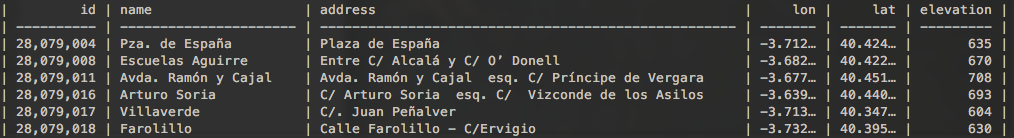
After unzipping the dataset, you'll see a stations.csv that looks like:
You'll also see a file called csvs_per_year.zip. Unzip this too.
Now, in the csvs_per_year folder, there is one file per year. we'll use just 2001 madrid_2001.csv

Data in an xyz space should always have geometry information. In this case, we want every station's hourly pollution measurement to be a datapoint. Since the station is referenced by id in madrid_2001.csv, we will have to join this file with stations.csv to get that coordinates of the measurement in the same row.
We could write a script to do this operation, but since this is a common task, we'll use an off the shelf tool called csvkit to do this operation. csvkit is a collection of command line tools to process csvs.
To install csvkit, you need to have Python and pip installed. (pip, the Python package manager, usually comes installed if you already have Python installed.)
Then you can install csvkit with this command: sudo pip install csvkit
Here is more documentation about installing csvkit, if you have any trouble: 1) installing csvkit 2) tips and troubleshooting
If you have a lot of trouble installing csvkit, you can skip it and download the pre-processed output data at the bottom of this step.
csvkit can do things like cut up, merge and view csvs. For example, to generate the views of the csvs above, we can use the csvlook command provided in csvkit.
head csvs_per_year/madrid_2001.csv | csvlook
To merge the sensor data and the station data, we'll use the csvjoin command:
csvjoin -c "station,id" --left csvs_per_year/madrid_2001.csv stations.csv > out.csv
This merge might take a while. Be patient.
After the merge, you should see the merged table in out.csv
In case you had any trouble installing csvkit or doing the merge, we've provided a pre-processed copy of the output file here: https://github.com/stamen/here-xyz-demo/blob/master/urban-air-leaflet/out.csv
One of the most powerful features of XYZ is the ability to use tags to select features. In this tutorial we will use the command line tool to add tags while we upload our data.
Once you have the command line tool installed, you'll need to run here configure set to set up your credentials. Specifically, you'll need your App ID and App Code.
Now we're going to upload the air quality data using the command-line to add the appropriate tags. Before we upload any data, we need to create an empty XYZ space. Here's how we do that, adding a name and description:
here xyz create --title "urban-air" --message "urban air quality data uploaded from the command line"
You'll see the response:xyzspace '[SpaceID]' created successfully
Instead of "[SpaceID]", you'll see an eight-character string of numbers and letters. This is your SpaceID.
Take note of that ID. We'll need to use that for pretty much everything else we do.
Now try here xyz list to list all your XYZ spaces. You should see the one you just created, and any other spaces you have set up already.
You can also try here xyz describe [SpaceID] to get some details about any of your spaces.
Now we can upload some data. There are a few different flags you can include when uploading data, but the one we're most interested in right now is -p (or --ptag does the same thing). The -p flag lets us specify some properties in our GeoJSON file that we'd like to convert into XYZ tags. Since we want to be able query the data based on the time, we will tag every datapoint with it's hourly timestamp. The here CLI tool makes this easy with the property tag command:
here xyz upload -f out.csv --lat lat --lon lon --ptag date [spaceID]
The -p or --ptag will create tags from the GeoJSON properties.
To verify that the data has been populated, we can preview it with the show command, using the -w flag. This will open up a web browser tab with a map preview of your data:
here xyz show -w [spaceID]
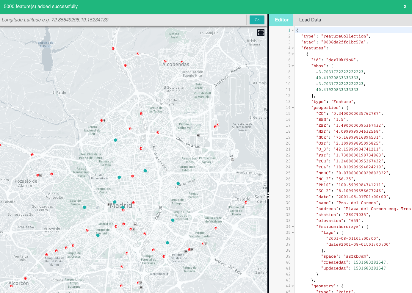
Notice the URL will look something like this:
http://geojson.tools/index.html?url=https://xyz.api.here.com/hub/spaces/[SpaceID]/search?limit=5000&access_token=[AccessToken]
In the data editor of this preview window, you should see that the properties object of each feature, there is a section for tags:
        "@ns:com:here:xyz": {
          "tags": [
            "2001-08-01t01:00:00",
            "date@2001-08-01t01:00:00"
          ],
          "space": "sZZXbJam",
          "createdAt": 1531683282547,
          "updatedAt": 1531683282547
        }
In this case the timestamp of the measurement has been turned into a tag.
The xyz api provides the ability to filter a dataset by tag. To try this out, use the geojson viewing tool and change the data provider url
from
http://geojson.tools/index.html?url=https://xyz.api.here.com/hub/spaces/[SpaceID]/search?limit=5000&access_token=[AccessToken]
to
http://geojson.tools/index.html?url=https://xyz.api.here.com/hub/spaces/[SpaceID]/search?limit=5000&access_token=[AccessToken]&tags=2001-08-01t01:00:00
(Basically, we just add &tags=2001-08-01t01:00:00 to the end of our URL.) If you then reload the page, the previewer re-renders with only data that matches data =='2001-08-01t01:00:00'
The map won't look very different, because the locations of the air quality sensors remain the same. But if you click on one of the dots to view the air quality results at that point, you can see that the date has changed and the values are different.
Try changing the date tag in the URL and reloading the page to get different data. For example, instead of 2001-08-01t01:00:00 (which is August 1st, 2001) try 2001-10-01t01:00:00 to see the data for October 1st.
Next, we will view some of this data in Leaflet. Leaflet is a simple mapping library that can draw simple points, lines, and polygons on top of a raster basemap.
Below we provide the code for a basic Leaflet template which gives us a raster "slippy" map, with nothing on it. You can either download the file index-step1.html and rename it to index.html, or you can create a new file called index.html in the text editing program of your chose, and copy-and-paste the code below.
Once you have your index.html file ready, let's see what it looks like. To view this code in your browser, you can quickly run a webserver using python -m SimpleHTTPServer. Or you could upload it to your own personal webpage, or use something like S3 or blockbuilder.org to view this simple page.
<!doctype html>
<html lang="en-us">
  <head>
    <meta charset="utf-8">
    <meta http-equiv="Content-Type" content="text/html; charset=utf-8">
    <meta name="viewport" content="width=device-width, initial-scale=1.0, maximum-scale=1.0, user-scalable=no">
    <title>Madrid Urban Air Quality</title>
    <link rel="stylesheet" href="https://unpkg.com/leaflet@1.3.3/dist/leaflet.css" />
    <link rel="stylesheet" href="https://cdn.jsdelivr.net/npm/flatpickr/dist/flatpickr.min.css">
    <script src="https://cdn.jsdelivr.net/npm/flatpickr"></script>

    <style>
        body {
            font-family: sans-serif;
            margin: 0px;
            border: 0px;
            padding: 0px;
        }
        .container {
            top: 0;
            left: 0;
            right: 0;
            bottom: 0;
            position: absolute;
        }
        .header {
            position: absolute;
            top: -8px;
            left: 0px;
            padding-left: 50px;
            right: 0;
            padding: 10px;
            z-index: 1000;
            background-color: rgba(255,255,255,0.75);
        }
        h2 {
            margin: 10px 0;
            margin-left: 50px;
        }
        h3 {
            margin: 0;
        }
        #map {
            height: 100%;
            width: 100%;
        }

        #property-list, #playback {
            display: inline-block;
        }

        .view {
            display: inline-block;
            font-size: 12px;
            border: 1px solid black;
            border-radius: 3px;
            margin: 3px;
            padding: 4px;
            background: #ffab96;
        }

        .view:hover {
            background: dodgerblue;
            color: white;
            margin-top: -2px;
            box-shadow: 1px 1px 1px black;
        }

        .view:active {
            margin-top: -2px;
        }

        #playback {
            margin-right: 1em;
            margin-left: 1em;
        }

        #playback .view {
            background-color: #ab96ff;
        }

        .view.selected {
            background: white;
            color: black;
        }

        #datepicker {
            margin-left: 50px;
            font-size: 12px;
        }

        .flatpickr-minute {
            pointer-events: none;
        }

        .flatpickr-minute + .arrowUp {
            pointer-events: none;
        }

        .flatpickr-minute + .arrowUp + .arrowDown {
            pointer-events: none;
        }

        .numInputWrapper:nth-child(3):hover {
            background: none;
        }

        .numInputWrapper:nth-child(3):hover .arrowUp {
            display: none;
        }

        .numInputWrapper:nth-child(3):hover .arrowDown {
            display: none;
        }


    </style>
  </head>

  <body>
    <div class="header">
        <h2>Madrid Urban Air Quality</h2>
    </div>
    <div class="container">
        <div id="map"></div>
    </div>

    <!-- leaflet -->
    <script src="https://unpkg.com/leaflet@1.3.3/dist/leaflet.js"></script>

    <!-- D3 -->
    <script src="https://d3js.org/d3.v5.min.js"></script>

    <!-- Demo setup -->
    <script>
        var theMap = L.map('map', {maxZoom: 14});
        theMap.attributionControl.addAttribution('Map tiles by <a href="http://stamen.com">Stamen Design</a>, under <a href="http://creativecommons.org/licenses/by/3.0">CC BY 3.0</a>. Map data by <a href="http://openstreetmap.org">OpenStreetMap</a>, under <a href="http://www.openstreetmap.org/copyright">ODbL</a>');

        L.tileLayer('http://tile.stamen.com/terrain/{z}/{x}/{y}.png').addTo(theMap);
        // center of madrid
        theMap.setView([40.416232, -3.703637], 13);

    </script>

  </body>
</html>
Admire your map! It should look like this:
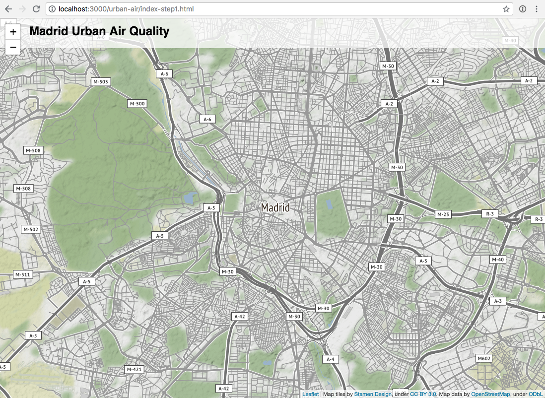
Now it's time to get some data on it!
We will load a GeoJSON layer from our XYZ space like so: https://xyz.api.here.com/hub/spaces/[SpaceID]/search?access_token=[AccessToken]&tags=2001-08-01t01:00:00
Note that we have to include a date tag filter, or else we will see hundreds of points stacked on top of each other at each air quality station.
So let's extend our code to load that data and to draw some circles on our map.
First, add this code at the very beginning of our script, before the line var theMap = L.map('map', {maxZoom: 14});:
        var circles = [];
        var initDate = '2001-02-23t09:00:00';
        var timeFormatter = d3.timeFormat('%Y-%m-%dt%H:%M:%S');
        var numberFormatter = d3.format(".1f");

        var properties = [
            { code: 'BEN', desc: 'benzene level measured in μg/m³' },
            { code: 'CO', desc: 'carbon monoxide level measured in mg/m³' },
            { code: 'EBE', desc: 'ethylbenzene level measured in μg/m³' },
            { code: 'MXY', desc: 'm-xylene level measured in μg/m³' },
            { code: 'NMHC', desc: 'non-methane hydrocarbons level measured in mg/m³' },
            { code: 'NO_2', desc: 'nitrogen dioxide level measured in μg/m³' },
            { code: 'NOx', desc: 'nitrous oxides level measured in μg/m³' },
            { code: 'OXY', desc: 'o-xylene level measured in μg/m³' },
            { code: 'O_3', desc: 'ozone level measured in μg/m³' },
            { code: 'PM10', desc: 'particles smaller than 10 μm' },
            { code: 'PXY', desc: 'p-xylene level measured in μg/m³' },
            { code: 'SO_2', desc: 'sulphur dioxide level measured in μg/m³' },
            { code: 'TCH', desc: 'total hydrocarbons level measured in mg/m³' },
            { code: 'TOL', desc: 'toluene (methylbenzene) level measured in μg/m³' }
        ];
        var currProperty = 'PM10';
All of that is just to help us parse the dates and to display descriptions for the various air quality indicators.
Next, add this code add the end of our script, basically all after the line theMap.setView([40.416232, -3.703637], 13);
        var spaceID = [SpaceID];
        var accessToken = [AccessToken];
        var radiusScale = d3.scaleLinear().domain([0, 200]).range([7, 70]).clamp(true);
        var colorScale = d3.scaleSequential(d3.interpolateOrRd).domain([0, 100]);
        function renderCircles() {
            // remove old markers
            circles.forEach(function (c) { c.remove(); })
            circles = [];

            theData.features.forEach(function (feature) {
                var c = L.circleMarker(
                    [feature.geometry.coordinates[1], feature.geometry.coordinates[0]],
                    {
                        radius: radiusScale(feature.properties[currProperty]),
                        // color: colorScale(feature.properties[currProperty]),
                        color: 'black',
                        fillColor: colorScale(feature.properties[currProperty]),
                        fillOpacity: 0.5
                    });
                c.addTo(theMap);
                c.bindTooltip('<h3>' + feature.properties.name + '</h3>' + '<b>' + currProperty + ': </b>' + numberFormatter(feature.properties[currProperty]) + '<br>' + properties.filter(d => d.code === currProperty)[0].desc);
                circles.push(c);
            });
        }

        function fetchData(dateStr) {
            var url = 'https://xyz.api.here.com/hub/spaces/' + spaceID + '/search?limit=100&access_token=' + accessToken + '&tags=' + dateStr;
            d3.json(url).then(function(data) {
                theData = data;
                renderCircles();
            });
        }

        fetchData(initDate);
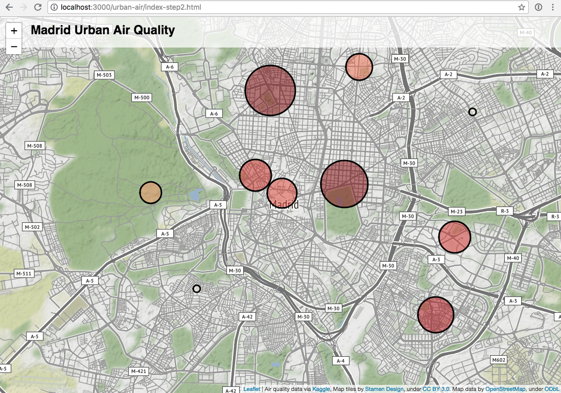
In this block of code, we're actually using d3.js to calculate appropriate circle sizes, but we're still using Leaflet to draw the circles on the map.
Note that we also add a tooltip to the circles, so you can see the raw data when you hover over a circle on the map.
At the end of this block of code, you can see the fetchData() function which is where we query the XYZ API to get the data.
Now your map should look something like this:
Next we will add some interactivity...
Each record returned by our XYZ query includes several different air quality measurements. Let's add some simple selection buttons so our user can view the different values in our data.
First add a new HTML element after the line <h2>Madrid Urban Air Quality</h2>
<div id="property-list"></div>
This div is where our buttons will go.
Now, after we define our properties object (specifically, after the line var currProperty = 'PM10';) we will add a new function that will draw selection buttons for each air quality metric. When clicked, each button will re-render the circles using the new selected metric.
        function renderProperties() {
            var pp = d3.select('#property-list').selectAll('.view').data(properties);
            pp.enter()
                .append('div')
                .classed('view', true)
                .on('click', d => {
                    currProperty = d.code;
                    renderProperties();
                    renderCircles();
                })
                .attr('title', d => d.desc)
                .text(d => d.code)
                .merge(pp)
                .classed('selected', d => d.code === currProperty);
        }
Finally, at the end of our script, we call this function once to draw the buttons:
renderProperties();
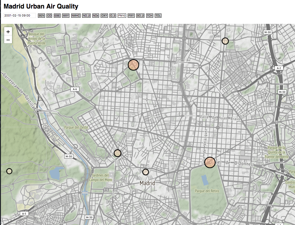
Now your map should look something like this:
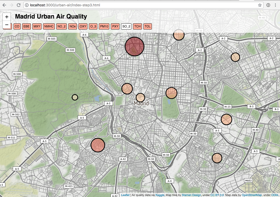
Try clicking on the different buttons to see the circles change size!
This interactivity is pretty cool, but we're only viewing different aspects of the data that we've already downloaded. Now let's let the user select data for a different date, which will trigger a new XYZ query and use our XYZ tags to download the correct data.
We're going to use the flatpickr library, which we already included in the header of our html page. Now, after the line <h2>Madrid Urban Air Quality</h2>, let's add an input for our date picker control:
<input id="datepicker" class="flatpickr flatpickr-input" type="text" placeholder="Select Date..." readonly="readonly">
And then in our script, we need to call the flatpickr function to create the control itself:
        var calendar = flatpickr("#datepicker", {
            enableTime: true,
            dateFormat: "Y-m-d H:i",
            minDate: "2001-01-01",
            maxDate: "2001-12-31",
            minuteIncrement: 60,
            onChange: function(selectedDates, dateStr, instance) {
                fetchData(timeFormatter(selectedDates[0]))
            }
        });
Notice how the date picker will call the fetchData() function anytime the user changes the currently-selected date. If you recall, fetchData() makes a query to XYZ using the requested date tag, and then re-renders the circles with the new data.
Finally, we need need to add one more line to populate our date picker with the initial date:
calendar.setDate(initDate);
Your map should now look like this:
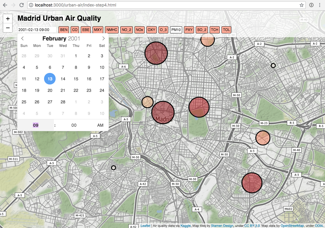
Click on the date to open up the calendar interface, and try choosing different dates or times to see the map update!
The date picker is pretty powerful, because it lets us select any date we choose. However, it's a bit inconvenient if we simply want to watch how the data changes over time. For our final enhancement, let's add a play button.
After the datepicker <input> element, add these lines:
<div id="playback">
<div id="back" class="view" onclick="addHours(-1)"><</div>
<div id="play" class="view" onclick="play()">Play</div>
<div id="next" class="view" onclick="addHours(1)">></div>
</div>
These buttons will make it easy to move forward or backward one hour at a time. Now in our <script> tag, add the appropriate functions and variables:
        function addHours(n) {
            var selectedDate = calendar.selectedDates[0];
            selectedDate.setHours(selectedDate.getHours() + n);
            calendar.setDate(selectedDate, true);
        }

        var playTimer;

        function play() {
            if (playTimer) {
                window.clearInterval(playTimer);
                playTimer = 0;
                document.getElementById("play").innerHTML = "Play";
            } else {
                playTimer = window.setInterval(function() { addHours(1) }, 1000);
                document.getElementById("play").innerHTML = "Pause";
            }
        }
Now if we reload our map, we should see this:
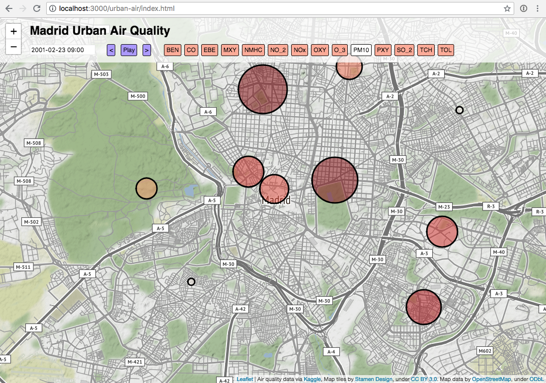
Try out the "play" button, or the forward/backward arrows. Each time the map switches to a new date, it is making a new query to XYZ, using on the tags that you created when you uploaded the data. Pretty cool, right?